Outline:

• prosthaphaeresis formulas

• averaging out components to remove them

• integration against a test function

• finding frequencies in an audio file

• frequency components as an alternative representation of a function

Week – : Finding the components of a measured signal

In a previous lab, we showed how to rewrite the complicated function

\[ f(t) = 3\sin(2\pi220t) -\cos(2\pi220t)+\sin^2(2\pi220t)+2\sin(2\pi440t+\pi/6) \]

using just two sinusoid components,

\[ f(t) = \sqrt{10} \sin(2\pi 220 t-\arctan(1/3)) +\frac{1}{2} + \frac{\sqrt{13}}{2}\sin\left(2\pi 440 t+\arctan\left(1/2\sqrt{3}\right)\right). \]

We frequently want to recover the components of a sound in this way, but usually we are not so lucky as to have an explicit functional form written out. Instead, we have measurements of the function at regular intervals. If we just had a measurement of the sound, using a digital microphone perhaps, how would we figure out what sound components make up that signal?

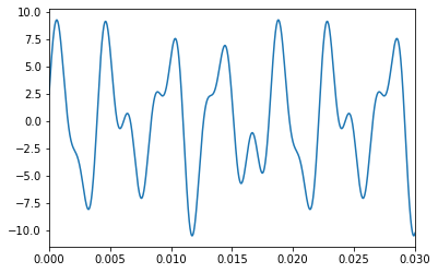
The following cell loads and plots a function sampled at 44100 Hz, for 5 seconds, consisting of three sine functions with frequencies 220, 330, and 495 Hz. We wish to uncover their amplitudes and phases. That’s the focus of this lab.

import numpy as np
import matplotlib.pyplot as plt

t = np.linspace(0, 5, 5*44100, endpoint = False)

#REMOVE THIS BEFORE GIVING TO STUDENTS
#x = 6*np.sin(2*np.pi*220*t+np.pi/4) + 2*np.sin(2*np.pi*330*t-np.pi/3) + 3*np.sin(2*np.pi*495*t)
#np.save('sampling_example.npy', x)

f = np.load('sampling_example.npy')
plt.plot(t, f)
plt.xlim(0, 0.03)
plt.show()

The prosthaphaeresis formula

We will use two powerful trig identities to make short work of this problem. In the early 1600s, before logarithms were invented, people would routinely use these formulas to compute products of numbers using tables of sines and cosines. This process was called prosthaphaeresis. That’s why I call it these the prosthaphaeresis formulas.

\[\begin{align*} \sin(a)\sin(b) &= \frac{1}{2} \cos(a-b)-\frac{1}{2}\cos(a+b)\\ \sin(a)\cos(b) &= \frac{1}{2} \sin(a-b)+\frac{1}{2}\sin(a+b) \end{align*}\]

We have a function \(f\) with a known form,

\[ f(t) = A \sin(2\pi 220t + a) + B \sin(2\pi 330 t+b) + C\sin(2\pi 495 t+c). \]

We wish to find the coefficients \(A\), \(a\), \(B\), \(b\), and \(C\), \(c\). We will exploit the prosthaphaeresis formulas by multiplying \(f\) by a known function.

\[\begin{align*} f(t)\sin(2\pi 220 t) &= A \sin(2\pi 220t + a)\sin(2\pi 220 t) + B \sin(2\pi 330 t+b)\sin(2\pi 220 t) + C\sin(2\pi 495 t+c)\sin(2\pi 220 t)\\ &= \frac{A}{2} \cos(a) - \frac{A}{2}\cos(2\pi 440 t+a) + \frac{B}{2}\cos(2\pi 110 t + b)- \frac{B}{2}\cos(2\pi 550 t +b) + \frac{C}{2}\cos(2\pi 275 t + c) -\frac{C}{2}\cos(2\pi 715 t + c) \end{align*}\]

the magic here is that one of these terms does not depend on \(t\) – it’s a constant. Let’s integrate the result across our entire sample period.

\[\begin{align*} \int_0^5 f(t)\sin(2\pi 220 t) \;dt &= \frac{A}{2} \cos(a) t - \frac{A}{4\pi 440}\sin(2\pi 440 t+a) + \frac{B}{4\pi 110}\sin(2\pi 110 t + b)- \frac{B}{4\pi 550}\sin(2\pi 550 t +b) + \frac{C}{4\pi 275}\sin(2\pi 275 t + c) -\frac{C}{4\pi 715}\sin(2\pi 715 t + c) \Big|_0^5\\ &= 5\frac{A}{2}\cos(a). \end{align*}\]

We multiplied by \(\sin(2\pi 220 t)\) which was carefully chosen so that all the terms involving \(B\), \(b\), \(C\), and \(c\) would disappear from the integral; those components complete a whole number of cycles over the domain, spending just as much time above the x-axis as below, so they all cancel out. This technique is called multiplying by a test function. We are testing our unknown function \(f\) by multiplying it by the “test function” \(\sin(2\pi 220 t)\).

Exercise

We just used one of the prosthaphaeresis formulas to show that

\[ \int_0^5 f(t)\sin(2\pi 220 t) \;dt = 5\frac{A}{2}\cos(a). \]

Use the other one to show that

\[ \int_0^5 f(t)\cos(2\pi 220 t) \;dt = 5\frac{A}{2}\sin(a). \]

Now that we have these, we can combine them. If we say \(X=5\frac{A}{2}\cos(a)\) and \(Y=5\frac{A}{2}\sin(a)\) then we must have

\[ X^2+Y^2 = \frac{25}{4} A^2. \]

Assuming \(A\) is positive, we can write \(A=\frac{2}{5}\sqrt{X^2+Y^2}\).

Exercise

In two or three sentences, explain why we can always assume \(A\) is positive and make up for the difference when picking the phase.

By taking the ratio \(Y/X\) we can cancel out \(A\), giving

\[ \frac{Y}{X} = \tan(a). \]

Taking the arctangent will get us exatly the value of \(a\). Actually, since the domain of arctangent is \((-\pi/2, \pi/2)\) but the phase could be anywhere, we can use the function arctan2 which takes a \(Y\) and and \(X\) value, and gives the angle to that point as a number between \(-\pi\) and \(\pi\). Let’s do that now, just instead of an integral we’ll use a Riemann sum.

X = (f * np.sin(2*np.pi*220*t)).sum()/44100
Y = (f * np.cos(2*np.pi*220*t)).sum()/44100
A = 2/5*np.sqrt(X**2+Y**2)
a = np.arctan2(Y, X)
print(A, a)

6.000000000000001 0.7853981633973324

There we have it: with some allowance for rounding errors, it looks like \(A\) is 6. We like to write phase a s a multiple of \(\pi\), so let’s divide that and see.

a/np.pi

0.2499999999999631

It looks like \(a\) has to be \(\pi/4\).

Exercise

The numbers we found were very close to \(6\) and \(pi/4\), but were off by a little bit. What could be causing this? Where did we lose a bit of precision?

Exercise

Find the amplitude and phase of each other component of \(f\). Give your best guess at the original numbers which were used to make \(f\), not just the approximation the computer gives you.

Exercise

What if we asked for the component of \(f\) at the frequency 440 Hz? What does this procedure give us? Have a go at it, and comment on the amplitude you find.

Generalizing this strategy

We have a pretty neat tool: if you provide a bunch of samples of a sinusoidal function, and specify what frequencies make it up, we can reconstruct the function exactly.

What if we apply this tool to a sound we found another way? I have made a recording of myself playing a chord on a melodica. Let’s listen to it now.

from scipy.io import wavfile
from IPython.display import Audio

rate, melodica = wavfile.read('melodica_recording.wav')

Audio(melodica, rate=rate)

Now, let’s use the same method we used above to get the frequency components. We learned previously that people aren’t sensitive to changes in phase of a sound, and can only hear sounds between 10 Hz and 20,000 Hz. So, let’s just try all the amplitudes for frequencies in that range. This may take a few minutes, since we have to do the whole integral 20,000 times. To save you some time, I have run the function below. It took about three minutes from start to finish.

from progressbar import progressbar

frequency = np.arange(10, 20_001)
def get_amplitudes(signal):
    t = np.arange(len(signal))/44100
    amplitudes = []
    for freq in progressbar(frequency):
        X = (signal * np.sin(2*np.pi*freq*t)).sum()
        Y = (signal * np.cos(2*np.pi*freq*t)).sum()
        A = 2/len(signal)*np.sqrt(X**2+Y**2)
        amplitudes.append(A)
    return np.array(amplitudes)

# I ran this code, taking 2 minutes 42 seconds.
# amplitudes = get_amplitudes(melodica)
# np.save('melodica_amplitudes.npy', amplitudes)

# you run this code instead:

amplitudes = np.load('melodica_amplitudes.npy')

What kinds of amplitudes do we get? Let’s plot it and see.

plt.plot(frequency, amplitudes)
plt.show()

We can see that a few frequencies really dominate the others. Which are they? Let’s pick an arbitrary threshold and inspect the five biggest amplitudes.

biggest = np.argsort(amplitudes)[:-6:-1]

import pandas as pd

pd.DataFrame({'frequency':frequency[biggest], 'amplitude':amplitudes[biggest]}).head()

	frequency	amplitude
0	443	1250.952284
1	1329	1149.409164
2	1328	922.722401
3	1571	739.491899
4	2005	491.903451

It makes sense that there is a significant amplitude at 443 Hz, because I was playing an F major chord which contains middle A. Down the line, the others are E, E again, G, and B.

What if we play all these notes together? What does that sound like?

reconstructed = np.zeros_like(melodica)
t = np.arange(len(melodica))/44100

# This takes about 90 seconds to run
#for f, a in zip(progressbar(frequency), amplitudes):
#    reconstructed = reconstructed + a * np.sin(2*np.pi*f*t)
#np.save('melodica_reconstructed.npy', reconstructed)

reconstructed = np.load('melodica_reconstructed.npy')

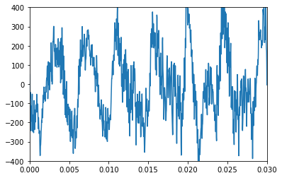
plt.plot(t, melodica, label='original recording')
plt.xlim(0, 0.03)
plt.ylim(-400, 400)
plt.show()
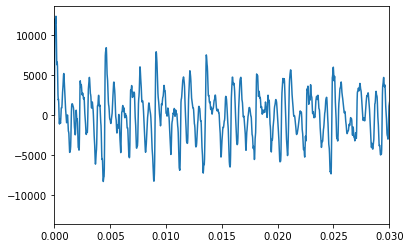
plt.plot(t, reconstructed, label='reconstructed from notes')
plt.xlim(0, 0.03)
plt.show()

Audio(reconstructed, rate=44100)

This sounds nearly the same as the sound we started with! The only weirdness is an audible beat pattern, with notes fading in and out. In a later lab, we will explore why this occurred.

Exercise

Below we load up a recording of a ukulele. Repeat the above procedure with that recording. What are the three loudest notes in the chord? How similar or dissimilar does it sound when you play back the notes?

rate, ukulele = wavfile.read('uke_recording.wav')

Audio(ukulele, rate=rate)

Conclusions

By using the technique of multiplying by test functions we were able to take a recording of sound and figure out exactly what phase and amplitude of sine waves went into it. This let us take a function and write it as a sum of sines, like so:

\[ f(t) = \sum_{k=100}^{20,000} A_k \sin(2\pi k t+a_k). \]

Even when we did not start with a signal made of pure sine waves, we were able to write a waveform this way and produce the same sound.

The list of amplitudes \(A_k\) is called the discrete Fourier transform of \(f(t)\). We can find the discrete Fourier transform of any waveform \(f\) to write it in terms of sines. When you write a function as a sum of sine functions in this way, it is called a Fourier series. In the following labs, you will learn:

• a much, much more fast and efficient way to compute the discrete Fourier transform

• how Fourier transforms are used to make MP3 files which are much, much more efficient at representing sounds

• more ways of representing a Fourier series, using complex numbers