Lab 1: Playing Sound#
Last updated May 7, 2024
00. Content #
Mathematics
Sinusoidal functions
Chromatic scale frequencies
Transformations of the independent variables: time reversal and time scaling
Programming Skills
Introduce the
Audiodisplay objectShow how to make sounds from a
numpyarrayManipulate audio as arrays:
concatenation
reversing
downsampling
upsampling
Embedded Systems
N/A
0. Required Hardware #
Headphones
Write your name and email below:
Name: me
Email: me @purdue.edu
What is a sound?#
Your ears are pretty remarkable. They are very sensitive air pressure sensors. When the air pressure fluctuates at frequencies within a certain range, sound waves are created. Through your ears, these sound waves are transformed into electric signals that your brain interprets as sound. These sound waves can be represented by functions (or, more generally, signals).
Let’s hear an example. If you have headphones, put them on now. Then, run the following cell and press play.
import numpy as np
from IPython.display import Audio
t = np.linspace(0, 5, 5 * 44100)
y = np.sin(440 * 2 * np.pi * t)
Audio(y, rate=44100)
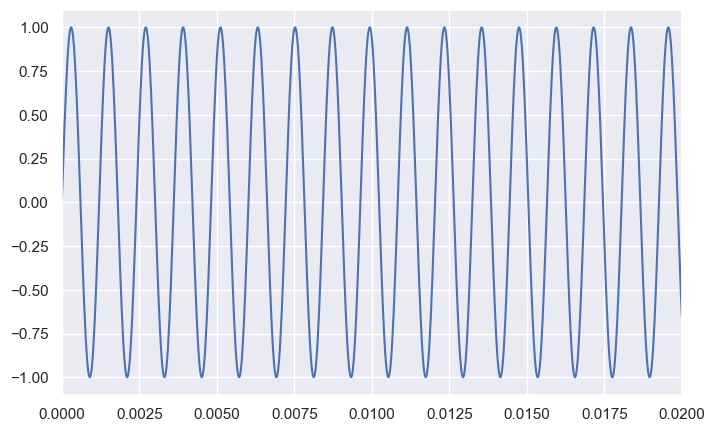
What did you just hear? Let’s visualize the sound wave function using a graph.
import matplotlib.pyplot as plt
import seaborn as sns
sns.set()
%matplotlib inline
plt.rcParams["figure.figsize"] = (8, 5)
fig, ax = plt.subplots()
ax.plot(t, y)
ax.set_xlim(0, 0.02)
plt.show()
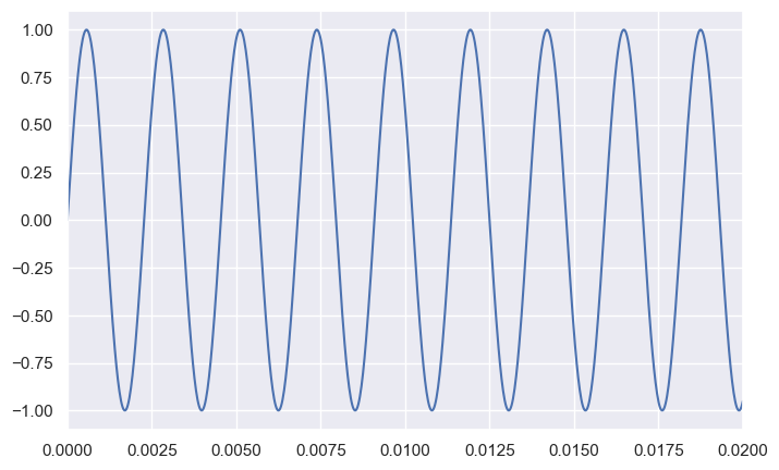
We can see that it is a sine wave with a frequency of 440 Hz. In music, the sound it makes is called A, or more specifically, A4 or “middle A”. When your ears detect air pressure changing in this pattern, you hear it as a middle A.
Let’s inspect the code we just used a bit more carefully. We gave the function Audio two parameters, y and rate. What’s in y?
y[:10]
array([0. , 0.06264861, 0.12505109, 0.18696228, 0.24813895,
0.30834076, 0.36733118, 0.42487847, 0.48075654, 0.53474585])
It’s a list of numbers showing the air pressure at various times. The scale of the y-axis is arbitrary, your computer re-scales it to make an appropriate volume before playing the sound. The parameter rate simply says how often to read a new number from the list. Most digital audio equipment is set up to read 44100 numbers per second, so that’s the rate we are using.
Exercise 1 #
Play an A 440Hz note for 3 seconds at a sampling rate of 44100Hz. Then Play an A 440Hz for 2 seconds at a sampling rate of 2000 Hz. (Jupyter doesn’t always play 2000 Hz properly. To confirm the autdio sounds correct, download the sound by clicking the three dots on the audio output object.)
Exercise 2#
Consider the function \(f(t)=sin(2\pi 400 t)\). What sound does it represent?
Exercise 3#
Consider the function \(f(t)=1+ sin(2\pi 400 t)\). What sound does it represent? Explain.
A more complicated sound#
The example above is quite simple, but you can actually make almost any sound this way. Let’s load up a more complicated sound, mystery_sound.txt and have a look at it.
mystery_sound = np.loadtxt("mystery_sound.txt")
fig, ax = plt.subplots()
ax.plot(mystery_sound)
ax.set_xlim(1000, 2000)
ax.set_ylim(-2000, 2000)
plt.show()
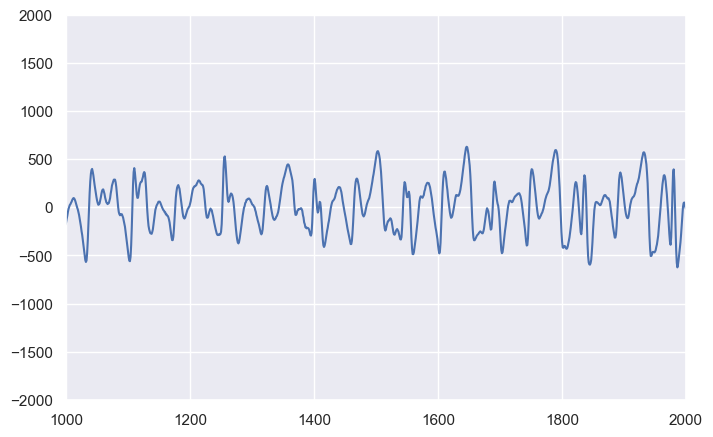
The curve it makes is not just a sine wave. What does it sound like?
Exercise 4 #
Use the Audio command to play this sound. Then, after listening to it, write down the name of the tune that plays.
Making sounds#
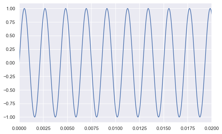
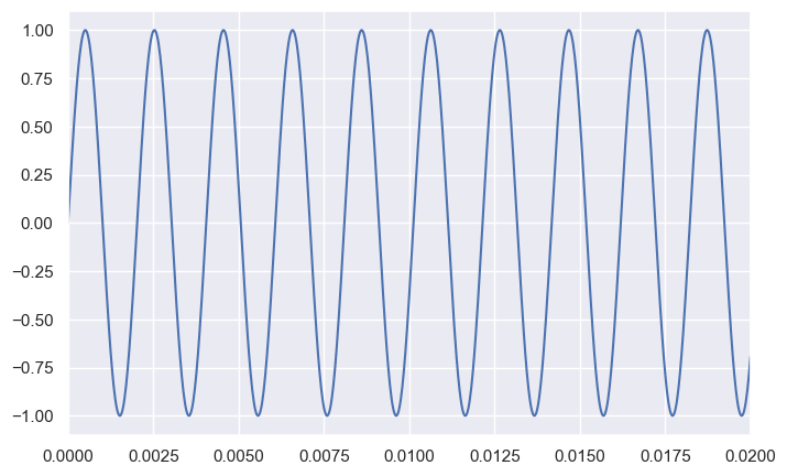
Now that you see a sound can be expressed as a list of numbers, let’s set about making our own music. We will need a way to make musical notes. To do that, we will use the chromatic scale. In the chromatic scale, an octave is a doubling of frequency. Also, twelve notes make up an octave and their frequencies are evenly spaced. These are the notes made by piano keys.
t = np.linspace(0, 0.5, 44100 // 2)
notes = "A A# B C C# D D# E F F# G G#"
frequencies = 440 * 2 ** (np.arange(12) / 12)
scale = dict(zip(notes.split(), frequencies))
for note, frequency in scale.items():
print("-" * 20)
print(f"Middle {note} has the frequency {frequency:.2f}")
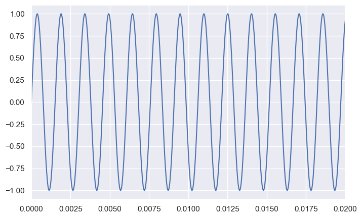
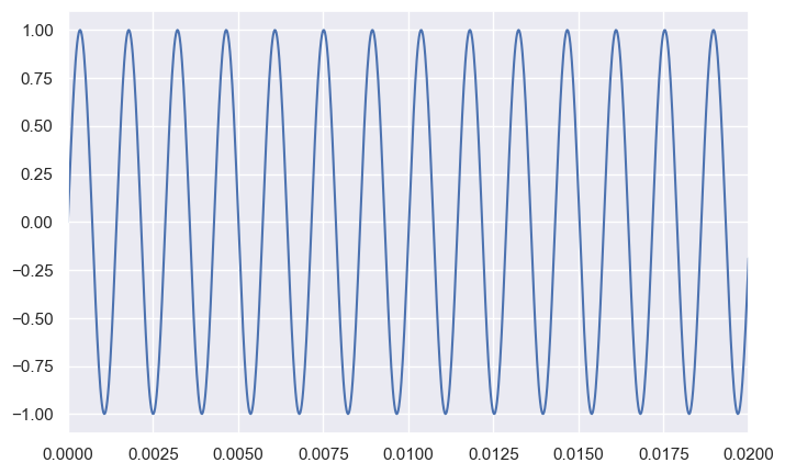
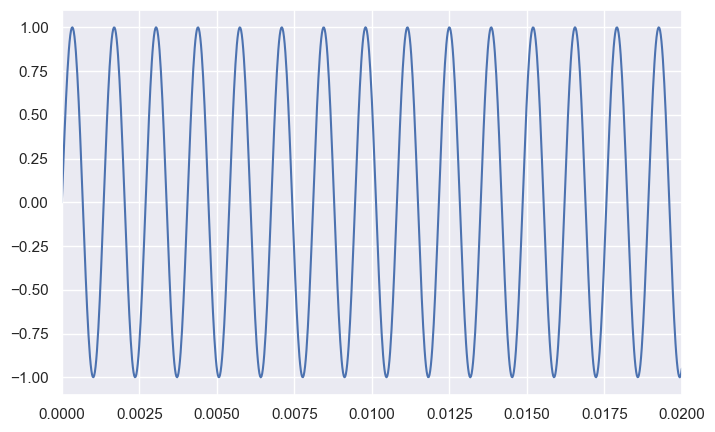
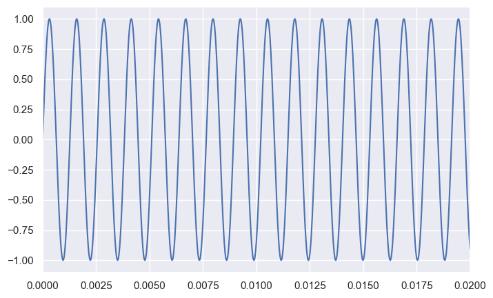
fig, ax = plt.subplots()
y = np.sin(2 * np.pi * frequency * t)
ax.plot(t, y)
ax.set_xlim(0, 0.02)
plt.show()
display(Audio(y, rate=44100))
--------------------
Middle A has the frequency 440.00

--------------------
Middle A# has the frequency 466.16
--------------------
Middle B has the frequency 493.88
--------------------
Middle C has the frequency 523.25
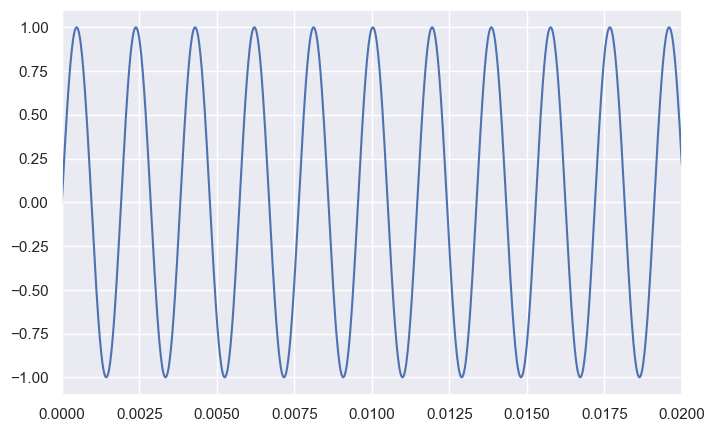
--------------------
Middle C# has the frequency 554.37
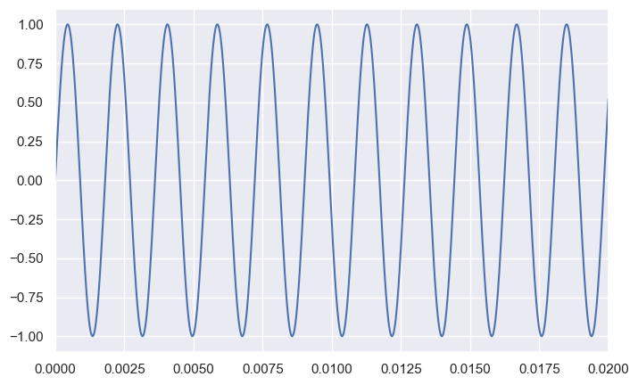
--------------------
Middle D has the frequency 587.33
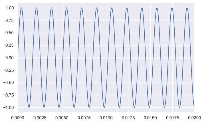
--------------------
Middle D# has the frequency 622.25
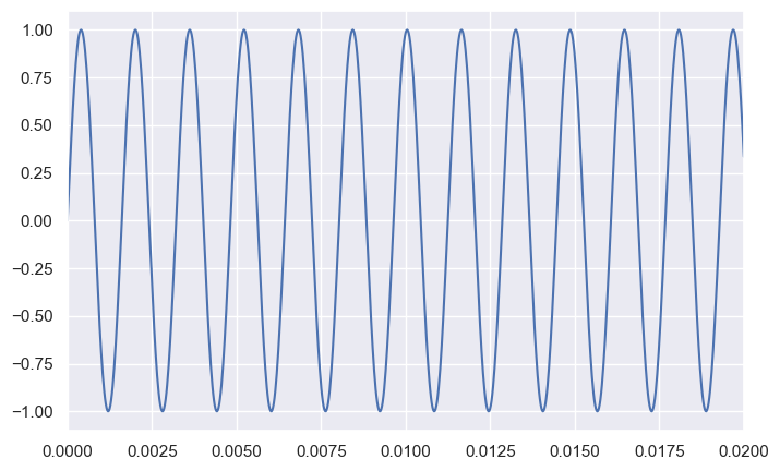
--------------------
Middle E has the frequency 659.26
--------------------
Middle F has the frequency 698.46
--------------------
Middle F# has the frequency 739.99
--------------------
Middle G has the frequency 783.99
--------------------
Middle G# has the frequency 830.61
By stringing these together, we can form a song. We will use the function np.concatenate which stacks up arrays end-to-end. Here is the start of “Row Row Your Boat”.
boat_notes = "C C C D E E D E F G"
boat_song = np.concatenate(
[np.sin(2 * np.pi * scale[note] * t) for note in boat_notes.split()]
)
print(boat_song[:10])
Audio(boat_song, rate=44100)
[0. 0.07448499 0.14855616 0.22180199 0.29381555 0.36419675
0.43255457 0.49850923 0.56169432 0.62175878]
Exercise 5 #
Play the C chord (i.e. C, E and G played together at the same time). Hint: Try adding the functions for each note.
Making Music#
Let us explore more about the audio array. What if we only play every other number? Let’s try it with slicing.
faster = boat_song[::2]
print(faster[:10])
Audio(faster, rate=44100)
[0. 0.14855616 0.29381555 0.43255457 0.56169432 0.67836891
0.77998911 0.86429975 0.9294298 0.97393389]
Now let’s try dragging the notes out longer by repeating each number twice.
slower = np.repeat(boat_song, 2)
print(slower[:10])
Audio(slower, rate=44100)
[0. 0. 0.07448499 0.07448499 0.14855616 0.14855616
0.22180199 0.22180199 0.29381555 0.29381555]
When we play it back faster, the song has a higher pitch but lasts half as long. When we play it back slower the song has a lower pitch and lasts twice as long. Most people find that the song is still recognizably the same when the pitch is doubled or halved, so we give a note with twice or one-half the frequency the same letter. Here is a wider scale we can use:
full_scale = {}
for i in range(1, 7):
for j, letter in enumerate(notes.split()):
full_scale[letter + str(i)] = 440 * 2 ** (i - 4 + j / 12)
full_scale
{'A1': 55.0,
'A#1': 58.27047018976124,
'B1': 61.7354126570155,
'C1': 65.40639132514966,
'C#1': 69.29565774421802,
'D1': 73.41619197935188,
'D#1': 77.78174593052023,
'E1': 82.4068892282175,
'F1': 87.30705785825097,
'F#1': 92.4986056779086,
'G1': 97.99885899543733,
'G#1': 103.82617439498628,
'A2': 110.0,
'A#2': 116.54094037952248,
'B2': 123.47082531403103,
'C2': 130.8127826502993,
'C#2': 138.59131548843604,
'D2': 146.8323839587038,
'D#2': 155.56349186104046,
'E2': 164.813778456435,
'F2': 174.61411571650194,
'F#2': 184.9972113558172,
'G2': 195.99771799087466,
'G#2': 207.65234878997256,
'A3': 220.0,
'A#3': 233.08188075904496,
'B3': 246.94165062806206,
'C3': 261.6255653005986,
'C#3': 277.1826309768721,
'D3': 293.6647679174076,
'D#3': 311.1269837220809,
'E3': 329.6275569128699,
'F3': 349.2282314330039,
'F#3': 369.9944227116344,
'G3': 391.99543598174927,
'G#3': 415.3046975799451,
'A4': 440.0,
'A#4': 466.1637615180899,
'B4': 493.8833012561241,
'C4': 523.2511306011972,
'C#4': 554.3652619537442,
'D4': 587.3295358348151,
'D#4': 622.2539674441618,
'E4': 659.2551138257398,
'F4': 698.4564628660078,
'F#4': 739.9888454232688,
'G4': 783.9908719634985,
'G#4': 830.6093951598903,
'A5': 880.0,
'A#5': 932.3275230361799,
'B5': 987.7666025122483,
'C5': 1046.5022612023945,
'C#5': 1108.7305239074883,
'D5': 1174.6590716696303,
'D#5': 1244.5079348883237,
'E5': 1318.51022765148,
'F5': 1396.9129257320155,
'F#5': 1479.9776908465376,
'G5': 1567.9817439269973,
'G#5': 1661.2187903197805,
'A6': 1760.0,
'A#6': 1864.6550460723597,
'B6': 1975.533205024496,
'C6': 2093.004522404789,
'C#6': 2217.4610478149766,
'D6': 2349.31814333926,
'D#6': 2489.0158697766474,
'E6': 2637.02045530296,
'F6': 2793.825851464031,
'F#6': 2959.955381693075,
'G6': 3135.9634878539946,
'G#6': 3322.437580639561}
Exercise 6 #
Here are the notes for the chorus of Hail Purdue. Play the song!
D#3 D#3 F3 G3 G#3 A#4 C4 C4 C#4 C#4 G#3 A#4 C4 C4 C4
Exercise 7 #
Write your own song, including some chord, play it, and save the data in a text file. Exchange your text file with someone else in the class.
Exercise 8 #
Play the file you received from your colleague once forward and once backward.
Exercise 9 #
Let f(t) be a function representing a sound wave. What function g(t) represents the sound wave played backward?
Exercise 10 #
Musicians often speed up or slow down their music for an artistic effect. The file chipmunk.txt has an excerpt from The Chipmunk Song by Ross Bagdasarian. Make a slowed-down version so you can hear what he sounded like while recording the voices of the chipmunks.
chipmunk = np.loadtxt("chipmunk.txt")
Audio(chipmunk, rate=44100)
Exercise 11 #
Let f(t) be a function representing a sound wave. What function \(g(t)\) represents the sound wave played twice as slow?
Reflection #
Do not skip this section! It will be graded but only on completion.
1. What parts of the lab, if any, do you feel you did well?
2. What are some things you learned today?
3. Are there any topics that could use more clarification?
4. Do you have any suggestions on parts of the lab to improve?
