Lab 10: Frequency Analysis with the DFT#
Last updated 8/13/24
00. Content #
Mathematics#
DFT
IDFT
Programming Skills#
FFT
IFFT
Embedded Systems#
N/A
0. Required Hardware #
N/A
Write your name and email below:
Name: me
Email: me @purdue.edu
1. Introduction #
In a previous lab, we covered how to sample real-time signals and learn the frequency components of the signal using Discrete Fourier Transform (DFT).
Recall that the DFT of a discrete-time signal with period \(N\), \(f_d[n]\) is defined as:
and the specific value of entry \(F[k]\) is called the k-th coefficients of the DFT of the signal and the DFT coefficient with the largest magnitude indicates the largest frequency contained in the signal.
DFT is a powerful tool in signal analysis with wide applications like reconstruction of medical images, computational photography, digital compression, noise cancellation in headphones, telecommunication and many more.
2. Denoising a Signal #
Let us consider that you are recording a person playing a piano in a mall using a basic audio recorder. Even if you are standing close to the audio source, it is wise to assume that the audio recorder will pick up the ambient noise and sound of other people in the busy mall. In such a case, we need a way to seperate the background noise from the music in the recording.
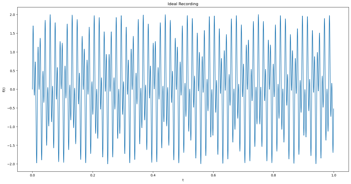
Let us consider a 1 second clip of the performance where the pianist played an \(A_1\) (55Hz) and \(B_2\) (123Hz) notes. Let us look at what the signal looks like in a perfect environment without any noise by loading ideal_piano_recording_example.npy.
import numpy as np
import matplotlib.pyplot as plt
from IPython.display import Audio

# the values used during the recording are provided
sampling_rate = 2100
sampling_period = 1/sampling_rate
duration = 1

t = np.arange(0, duration, sampling_period)


ideal_recording = np.load('ideal_piano_recording_example.npy')

Audio(ideal_recording, rate=sampling_rate)
# NOTE: if this doesn't play, click the three dots to download and play the audio
Now, let us plot and observe the ideal recording in time domain.
plt.figure(figsize = (18, 9))
plt.plot(t, ideal_recording)
plt.title('Ideal Recording')
plt.xlabel('t')
plt.ylabel('f(t)')
plt.show()
Now let us look at our noisy recording, noisy_piano_recording_example.npy and try to recover the original sound from it.
actual_recording = np.load('noisy_piano_recording_example.npy')
Audio(actual_recording, rate=sampling_rate)
# NOTE: if this doesn't play, click the three dots to download and play the audio
As expected, there is a discernible differnce between two audio samples. Now let us plot and visualize this recording.
plt.figure(figsize = (18, 9))
plt.plot(t, actual_recording)
plt.title('Actual Recording')
plt.xlabel('t')
plt.ylabel('f(t)')
plt.show()
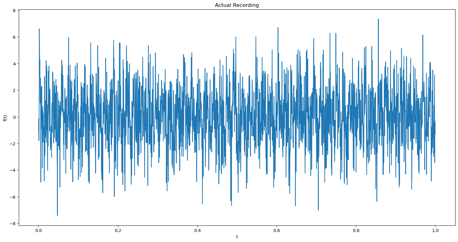
We can see that the time domain plots of both the signals are not distinguishable. So it is safe to assume that we cannot approximate the original signal from this time domain plot alone.
Let us see the frequencies contained in the recording by plotting its dft.
dft = np.fft.fft(actual_recording)
abs_dft = np.abs(dft)
num_samples = len(actual_recording)
xf = np.fft.fftfreq(num_samples, 1/sampling_rate)

plt.figure(figsize = (18, 9))
plt.stem(xf, abs_dft)
plt.xlim(-150, 150)
plt.title('DFT of Actual Recording')
plt.xlabel('frequency')
plt.ylabel('Amplitude')
plt.show()
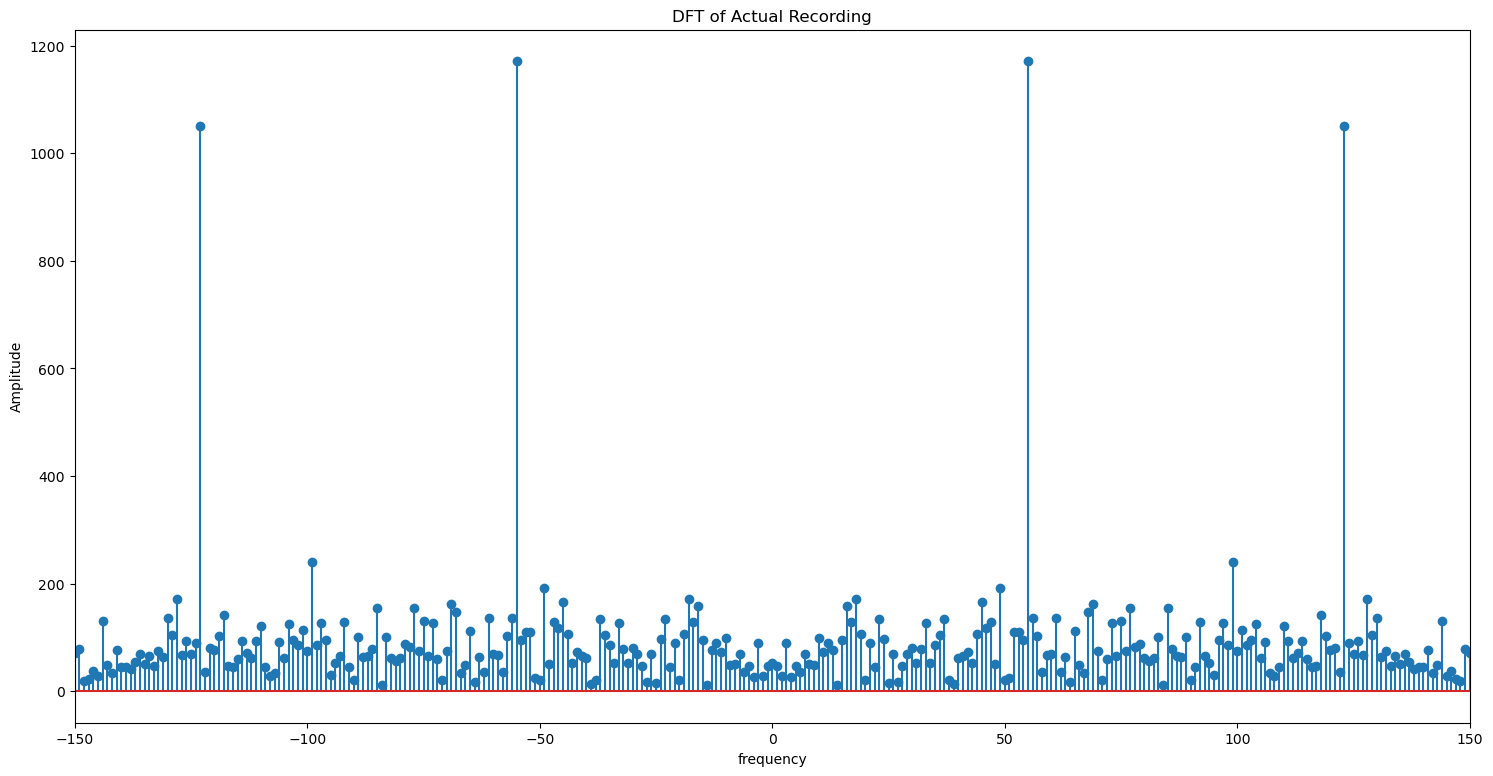
This DFT plot gives us an idea about the dominant frequencies in the signal. By looking at the amplitudes, we can identify that the dominant frequencies in the recording are 55Hz and 123Hz. We can conclude with sufficient confidence that the other frequencies may likely be due to the noisy environment as the amplitudes are low for those frequencies. But it may not always be the case.
Now let us filter the noise from our recording and plot its dft.
# the above snippet will return a list, with 1s in indices
# where amplitude > 300 and 0s in other places.
noise_indices = abs_dft>300

# filter out the amplitude values under 300
dft_clean = noise_indices * dft
plt.figure(figsize = (18, 9))
plt.stem(xf, np.abs(dft_clean))
plt.xlim(-150, 150)
plt.title('DFT of Filtered Recording')
plt.xlabel('frequency')
plt.ylabel('Amplitude')
plt.show()
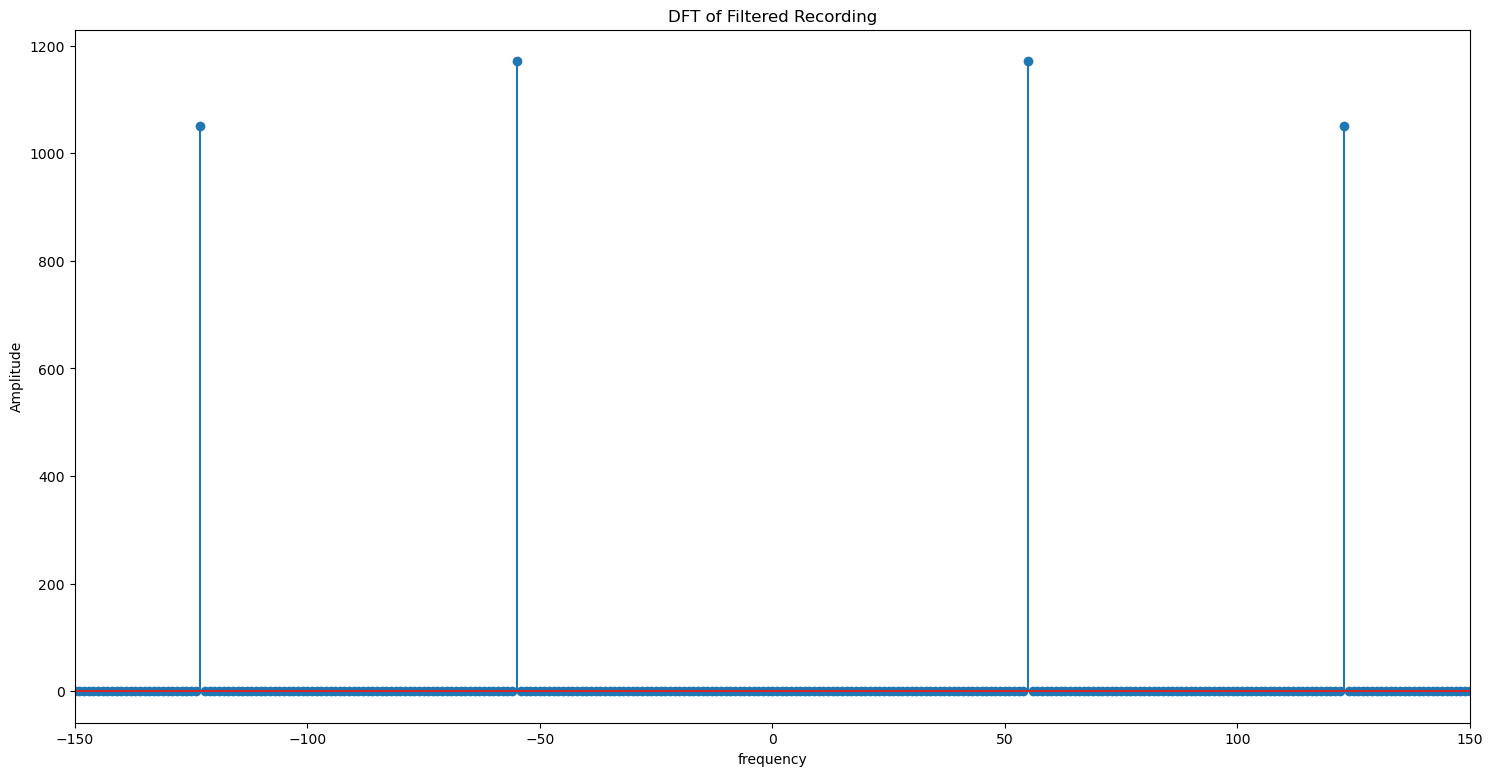
Let us compare this plot with the DFT of the ideal recording without any noise.
plt.figure(figsize = (18, 9))
plt.stem(xf, np.abs(np.fft.fft(ideal_recording)))
plt.xlim(-150, 150)
plt.title('DFT of Ideal Recording')
plt.xlabel('frequency')
plt.ylabel('Amplitude')
plt.show()
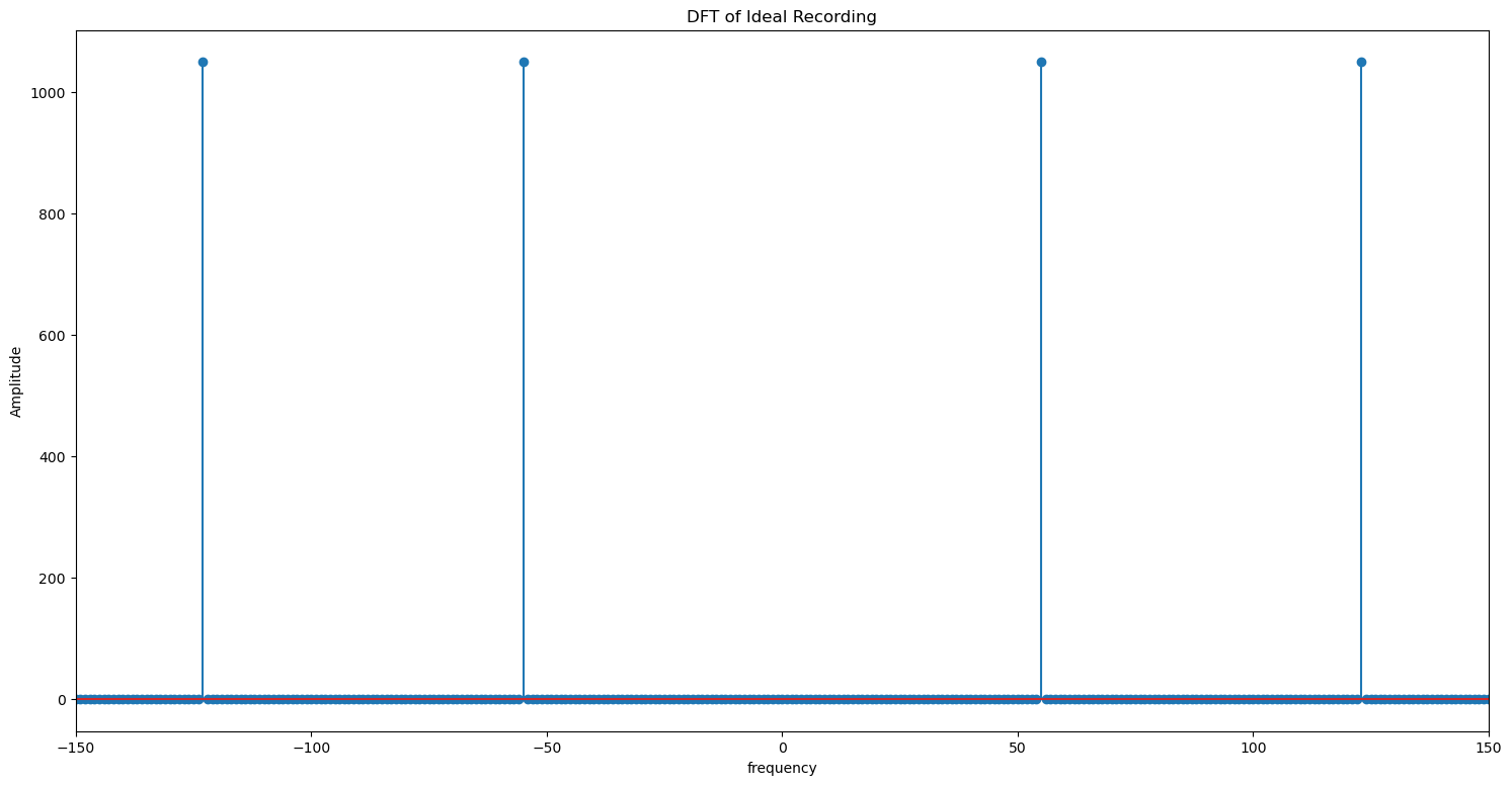
The filtered signal is identical to the original signal. We can now convert the denoised signal to time domain.
filtered_recording = np.fft.ifft(dft_clean)
Audio(filtered_recording, rate=sampling_rate)
C:\Users\elibo\anaconda3\lib\site-packages\IPython\lib\display.py:159: ComplexWarning: Casting complex values to real discards the imaginary part
  data = np.array(data, dtype=float)
# if getting: "ComplexWarning: Casting complex values to real discards the imaginary part"
if np.allclose(np.imag(actual_recording), 0): # check if all imaginary components are close to zero
    print("The array is all real.")
else:
    print("The array contains complex values.")

# The original signal is all real, so it is fine to discard the imaginary values.
# You can explicitly do this with np.real() and not get the warning:
filtered_recording = np.real(np.fft.ifft(dft_clean))
Audio(filtered_recording, rate=sampling_rate)
The array is all real.
plt.figure(figsize = (18, 9))
plt.plot(t, filtered_recording)
plt.title('Filtered Recording')
plt.xlabel('t')
plt.ylabel('f(t)')
plt.show()
C:\Users\elibo\anaconda3\lib\site-packages\matplotlib\cbook\__init__.py:1298: ComplexWarning: Casting complex values to real discards the imaginary part
  return np.asarray(x, float)
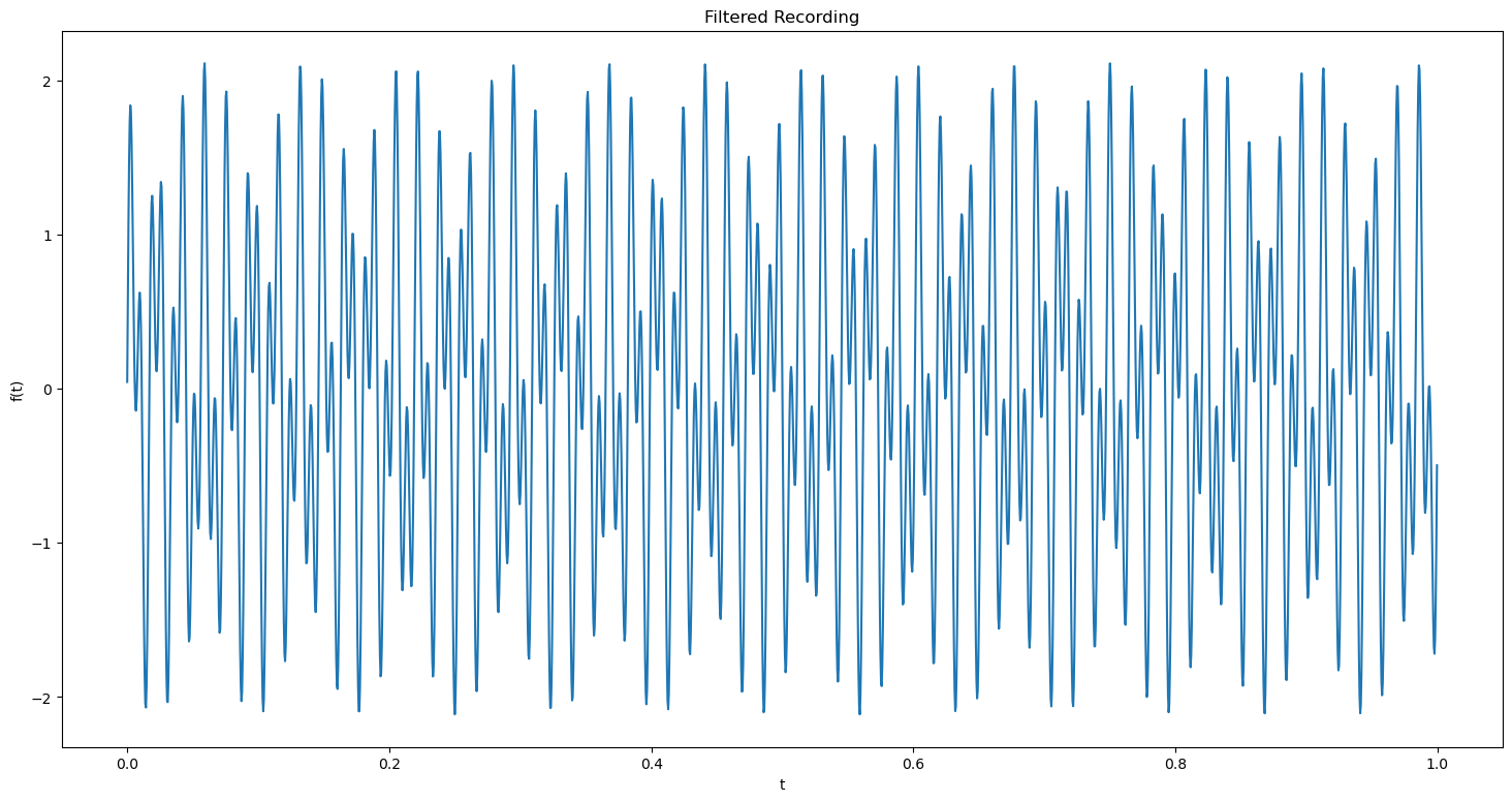
Note: We are clearly able to seperate the noise from the original signal due to the large difference between amplitudes of the frequencies. If the original signal and the ambient noise had the similar amplitude, we wouldnt be able to get a properly filtered signal.
Exercise 1 #
Build a signal that is a sum of sines of 5 different frequencies. Vary the magnitude of the coefficients so that one is very large compared to the others.
Play the sound corresponding to this signal.
Compute the DFT and plot their magnitude.
For what value of \(k\) is the magnitude of \(F[k]\) the largest? Denote this value of \(k\) by \(k_0\).
What frequency does the \(k_0\) you identified correspond to? Denote that frequency by \(f_0\).
Play the sound which only has the frequency \(f_0\). How does it compare to the original sound?
3. Determining the Dominant Frequency Components of a Signal #
Exercise 2 #
Load melodica_recording.wav and plot the recording.
Hint: load the file using scipy.io.wavfile.read and convert the file to a numpy array.
Play the sound corresponding to this signal.
Compute the DFT and plot its magnitude.
For what value of \(k\) is the magnitude of \(F[k]\) the largest? Denote this value of \(k\) by \(k_0\).
What frequency does the \(k_0\) you identified correspond to? Denote that frequency by \(f_0\).
Play the sound which only has the frequency \(f_0\). How does it compare to the original sound?
We can see that a few frequencies really dominate the others. Which are they? Let’s pick an arbitrary threshold and inspect the five biggest amplitudes.
Exercise 3 #
Keep the five most dominant frequencies from melodica_recording.wav and remove the rest. Plot its DFT and play the modified signal.
Exercise 4 #
Load up a recording of the ukulele, uke_recording.wav.
What are the dominant frequencies in this recording?
Remove frequencies with magnitude less than 500 from the recording.
Play the new sound and plot its DFT.
How does the new sound compare to the original?
Exercise 5 #
Use the voice recorder code from week 8 to record any song for a duration of 2 seconds.
Suppress the background noise in the recording.
Plot the amplitude and dft of the signals before and after denoising.
Play the modified signal.
Exercise 6 #
Modify the voice changer from week 8 to save the original and modified voice.
List the complete code here in a seperate code block.
Plot the amplitude and dft of both the signals.
Comment on the difference between the plots.
Reflection #
Do not skip this section! Assignment will be graded only on completing this section.
1. What parts of the lab, if any, do you feel you did well?
2. What are some things you learned today?
3. Are there any topics that could use more clarification?
4. Do you have any suggestions on parts of the lab to improve?
